Abstract
This website explores physical modelling synthesis of a plucked string combined with a reverberator to produce a range of ambient tones and drum timbres.
Introduction
Physical modelling synthesis incorporates the use of modern day computational power to model the complex physical characteristics and acoustics of real world sound. This includes musical instruments and audio effects. The fundamental design of physical models can be constructed by using Newton’s famous three laws of motion by the equation shown in figure 1.
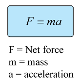
Figure 1 - Newton’s F = ma [1]
Due to the simplicity of Newtonian mechanics, simplifications have to be made conserving audio quality but reducing complexity and computational time. There are a wide range of physical-models and they use a combination of mathematical techniques as linked below [2].
Background
Karplus-Strong Algorithm
In 1983, Kevin Karplus and Alex Strong were students at Stanford University researching wavetable synthesis. They published a paper titled "Digital Synthesis of Plucked-String and Drum Timbres" [3] which outlined their experimentation of a new type of wavetable synthesis. They discovered that low-pass filtering the wavetable on every pass changed the timbre. As the name of the paper suggests, this sounded similar to a plucked string and was later developed into drums and wind instruments.
1D Wave Equation & Travelling Wave Solution
An ideal lossless string (shown in figure 2) can be solved for any string that is infinitely long.
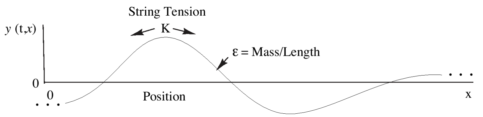
Figure 2 - Ideal Vibrating String. [4]
The pluck (regardless of shape) travels with a speed that is equal to the square root of spring tension divided by the mass over length of string. The equation is shown in figure 3.
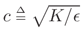
Figure 3 - String shape propagation speed in lossless ideal string [5]
The partial differential equation derived from this model was solved by d’ Alembert [6] to give a solution to a travelling 1D wave for a string:
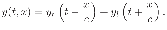
Figure 4 - Travelling Wave Solution. [7]
Assuming string slope is much less than 1, the solution is derived which demonstrates that y(t,x) can be represented by two wave functions. This shows that the physical state of a string can be converted to an equivalent pair of traveling components, one right and one left going (Yr and Yl respectively). Figure 5 depicts this in a plucked string.
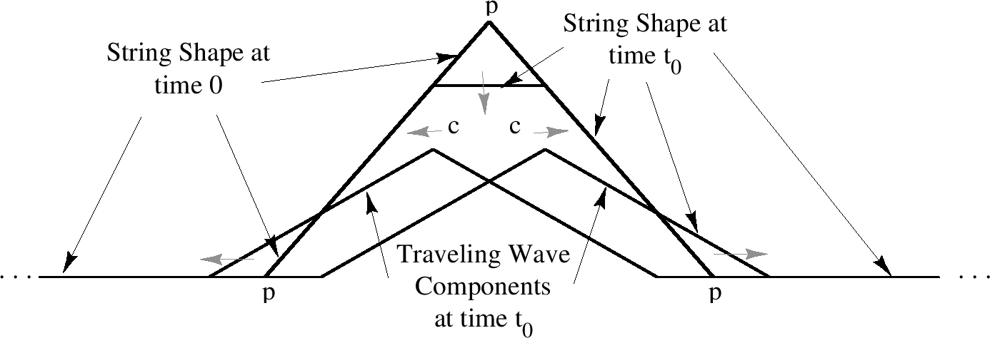
Figure 5 - Travelling Wave Components. [8]
In figure 5 we can visualise the traveling wave components. The string is plucked in the three points marked P giving it the initial shape. The pluck shape is then released and the top point at time 0 then starts to travel down and outwards at speed c. The actual wave shape can be considered as the sum of the two superpositioned smaller waves, as given in figure 4. In the real world we don't see this occur exactly, this is because we don't have an infinite string length and it is very difficult to pluck a perfectly shaped triangle. A visualization of the resultant wave is shown in figure 6.
Figure 6 - Resultant Wave Animation. [9]
Note: This simulation of the string is clamped either end and there is no dampening upon reflection, resulting in a perfect phase inversion. In reality, the oscillation would decay over time due to dampening characteristics of the string and its environment.
Digital Waveguide Model
d'Alembert's solution can be converted to digital delay lines by discretizing the 1D travelling wave solution. To do this, the travelling wave amplitude is sampled along the string and a sampling interval is defined. This means a digital waveguide model can be generated which provides a digital simulation of the travelling-wave solution. This is shown in figure 7.
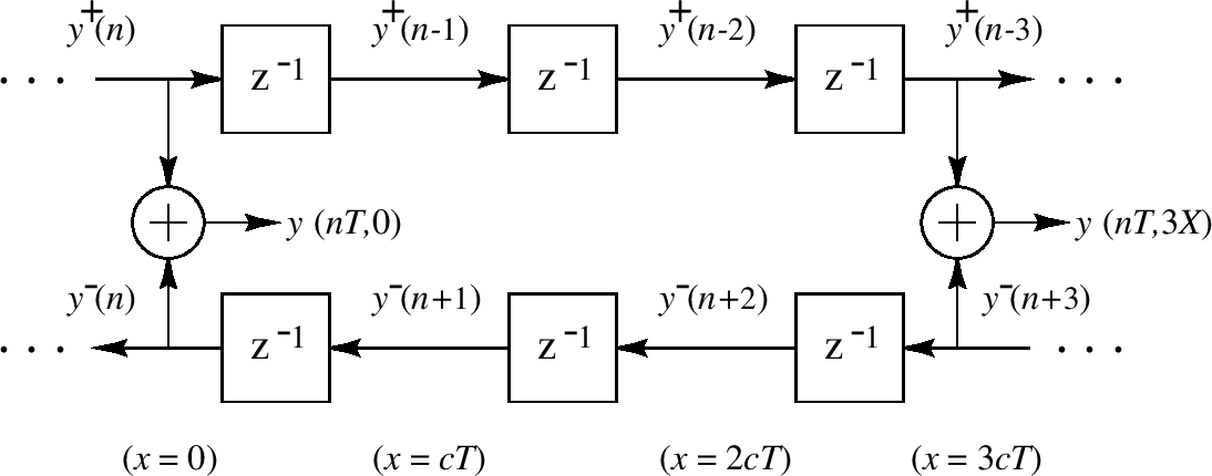
Figure 7 - Digital Implementation of a lossless waveguide system. [10]
Uses of Digital Waveguides
In the 1980s, there were many techniques used for digital music synthesis. These were methods such as frequency modulation, subtractive synthesis, additive synthesis and the use of wavetables. In 1983 Karplus and Strong explained that these synthesis techniques sounded rich but required large amounts of computational power [3]. Whereas, in comparison, algorithms which model a plucked-string can produce good quality sounds and use less arithmetic. It is worth noting that it is not a completely fair comparison, as the other synthesis techniques are more versatile and can produce a wider range of sounds, but computers weren’t powerful in 1983. In 1994, the plucked-string digital waveguide model was first commercially used in the Yamaha VL1 synthesiser [11]. This synthesizer used physical modelling to produce sounds that no one had really ever heard before at the time. Yamaha acknowledged their licensed use of Julius O. Smith’s work as base to produce the DSP (digital signal processing) chips within the synthesiser. Interestingly, Yamaha marketed the VL1 as ‘Virtual Acoustics’, which is their choice of renaming physical modelling. It is not clear why Yamaha did this. The VL1 is difficult to play and even more difficult to master. This is because the user is given a wide range of controls and physical models can be very sensitive to minor adjustments. However, if mastered, the VL1 was a high performing real-time synthesizer which could model acoustic instruments. Examples of the diverse range of sounds Yamaha developed are explored here:
Digital Waveguide Plucked String Model
The karplus-strong (KS) algorithm shown in figure 8 is a simplified digital waveguide synthesis model. It is used to model an ideal vibrating string with no stiffness and a defined dampening characteristic. The implementation loops the waveform around the signal chain and is modified by the filter each period. The dampening characteristic used by KS is a two-point moving average filter, this is shown as [1 + 1/Z]/2. It behaves as a first order low-pass filter.
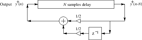
Figure 8 - Block Diagram of Karplus-Strong algorithm. [12]
The algorithm produces reasonable and somewhat realistic sounds of a string pluck. It is close to the sound of a guitar, but not completely realistic. A range of timbres can be produced through the manipulation of the pluck position, pickup and reflection coefficient.
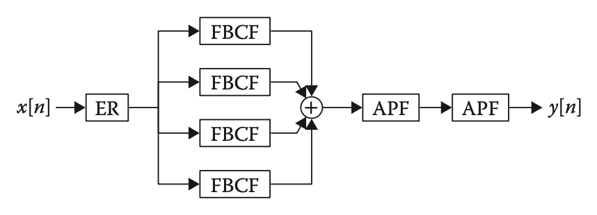
Moorer Reverberator
A reverberator imitates the acoustics of a natural space. Artificial reverb adds the impression of ambience to an acoustic signal that is ‘Dry’. We can create virtual spaces through the use of filtering algorithms. In the 1960s Schroeder introduced the concept of artificial reverb by connecting tapped delay lines to parallel comb filters passed into a series of all-pass filters. Tapped delay lines simulate the early reflections within a space. The parallel comb filters increase the density of the early reflections to produce a reverb tail. The allpass filters then simulate the final late reverb by increasing the density of reflections even more. In 1979, James Moorer developed Manfred Schroeder’s work by introducing a lowpass filter inside the comb filters [13]. The reverb is characterized by the comb filtering due to its uneven frequency response and the low pass filtering imitates the usual room acoustics of fast high frequency roll-off. This allows for frequency dependent reverb time control and results in a more natural sound. The design can be seen in figure 9.